

Code as Orca
Fourth in the series, and the first one about something that was never ours to simulate. Code as World ran a world. Code as Nature gave the lab a body. This one asks a smaller question with a harder edge on it: what is a whale call, written down? And once you can write one down, what does it take to say where the animal goes next? Ten cards. Every number on this page is output from the program in this repository. None of it is a whale.
Source: media/src/orca/orca.py (composition, step, the renderers) and gen.py (run it, write the cards). Stdlib only, no model in the loop, no network at render time, no audio file anywhere in the tree. Same seeds, same cards.
The line, drawn in the frame
This page has a failure mode the other three do not. Synthesised pictures of a real scientific object look like results. Put a confusion matrix on a page and it reads as a measurement no matter what the caption underneath it says, because visual grammar beats caption text every time. So there is no confusion matrix here, and the line between cited and invented is drawn inside the image rather than under it.
Two treatments, applied without exception. A solid sand edge with a credit strip means the card's content traces to published work, named on the card. A loud dashed edge with an ILLUSTRATIVE badge means this program made it up. The test is deliberately crude: blur the text and you can still tell which is which. The badge is rendered into the SVG, not added in HTML, so it survives a crop, a screenshot and a repost onto somebody else's timeline.
Two badges, not one, for the same reason. The Ornstein-Uhlenbeck credit names a specific published method, and naming a specific method is a credibility improvement and a risk increase in the same move — it sounds precise enough to be mistaken for the real thing. So that badge appears only on the four cards that actually illustrate the method. The other synthesised cards carry a plainer one that claims nothing.
10 cards — 4 call catalogue, 4 forecast, 2 bioacoustics; 2 carrying a credited source, 8 carrying the illustrative badge. Forecast: seed 3, 24 paths, 300 ticks of dt = 0.1 s (30 s), θ = 0.55, σ = 14, preferred cruise 42 px/s, heading blend 0.72/0.28. Ensemble spread 0 px at tick 0, 220.9 px at tick 300, with 2 of 24 paths ending inside the abstract hazard band. Calls: contour 101 against 102 at 0.1418 octaves, against 0 for a contour matched with itself; repertoire seed 7 gives 1 type shared by every group and 2 held by one. Naive detector: 33 calls caught, 30 false alarms of which 30 are boats, 8 missed, at threshold 0.62 over 160 synthetic events.A call is a shape
Killer whale pulsed calls fall into discrete types, and the types are countable — that is Ford's catalogue and it is why acoustic source identification is a tractable problem rather than a wish. A type is defined by the shape of its frequency contour over time: an onset sweep, a held plateau with a wobble in it, a terminal drop. Two calls are the same type when their contours sit on top of each other.
The four contours on this page are synthesised from fixed seeds. They are cartoons of the right kind of object, and the card that shows which groups use which types is constructed to be legible rather than sampled — a uniform draw kept producing a full grid, which states the opposite of what the card is about. The one honest number in the set is the distance measure: mean absolute separation in octaves between two contours, which is the arithmetic sitting underneath the intuition. A real classifier does far more, and HALLO's is a neural one.
A forecast is a spread, not a dot
The second half is movement. The natural family for an animal that keeps its momentum is an Ornstein-Uhlenbeck process on velocity rather than position: the animal is pulled back toward a preferred speed and heading, and noise pushes it off. Direction blending means the pull target is itself a blend of where the animal is already going and where the channel wants it to go. That is the shape of the method in Lin's 2023 SFU thesis, and the shape is all this page takes.
Twenty-four paths start from one point with one velocity. Nothing separates them except the noise term. What the frames show is the only output a forecast of this kind can honestly produce: not a line, but a widening cloud, with the spread as the error bar. The hazard card is why anyone builds one at all — but it is a circle on an empty field, not a channel, not a shipping lane, and not a map of anywhere. A real system outputs a probability over a real place. This is not one.
The step function, read from orca.py when the site was built:
def step(state, dt):
    """One Euler-Maruyama step of the O-U velocity process with direction blending."""
    for p in state["paths"]:
        vx, vy = p["vel"]
        speed = math.hypot(vx, vy)
        # --- direction blending: target heading is current heading blended with preferred ---
        cur = math.atan2(vy, vx) if speed > 1e-9 else state["prefer"]
        tx = W_PERSIST * math.cos(cur) + W_PREFER * math.cos(state["prefer"])
        ty = W_PERSIST * math.sin(cur) + W_PREFER * math.sin(state["prefer"])
        tn = math.hypot(tx, ty) or 1.0
        mux, muy = (tx / tn) * MU_SPEED, (ty / tn) * MU_SPEED
        # --- O-U on velocity: pull toward mu, plus a Wiener increment ---
        rt = math.sqrt(dt)
        vx += THETA * (mux - vx) * dt + SIGMA * rt * p["rng"].gauss(0.0, 1.0)
        vy += THETA * (muy - vy) * dt + SIGMA * rt * p["rng"].gauss(0.0, 1.0)
        p["vel"] = [vx, vy]
        p["pos"][0] += vx * dt
        p["pos"][1] += vy * dt
        # the frame is a channel, not a torus: reflect, so nothing teleports between frames
        # (the /world orca wrapped at tick 59 of 60 and hid the jump in the gap)
        for k, hi in ((0, W), (1, H)):
            if p["pos"][k] < 40:
                p["pos"][k] = 40.0; p["vel"][k] = abs(p["vel"][k])
            elif p["pos"][k] > hi - 40:
                p["pos"][k] = hi - 40.0; p["vel"][k] = -abs(p["vel"][k])
        p["trail"].append((p["pos"][0], p["pos"][1]))
    state["t"] += dt
    state["tick"] += 1
    return state
The set
Four on the call catalogue, four on the forecast, two on the bioacoustics. The captions are the program's own numbers, including the ones that make the work look bad: the naive detector card reports its false alarms rather than its accuracy, because a rule that fires on a passing boat is the lesson, and a score would have buried it.
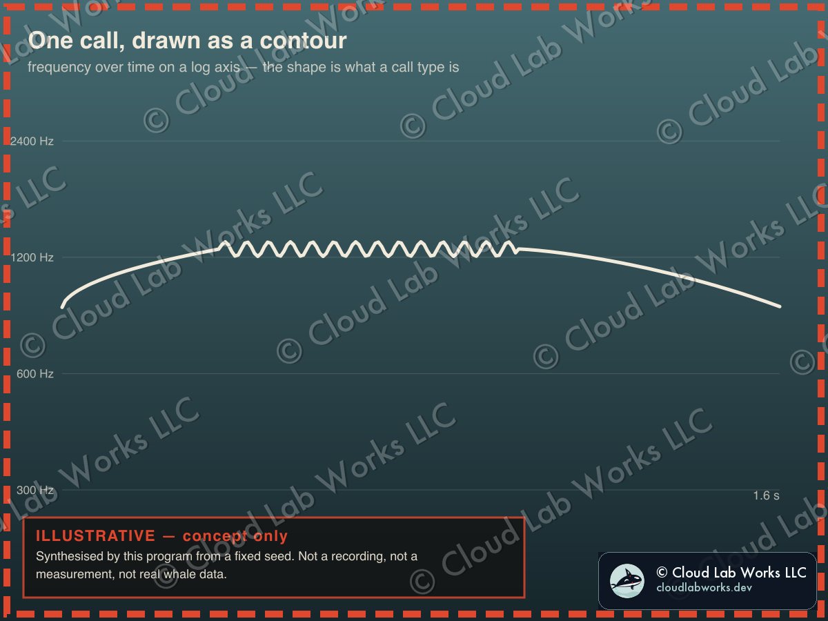 SVG · Call catalogue · illustrativeOne call, drawn as a contourOnset 891 Hz, plateau 1261 Hz with a 8.5 Hz wobble at 4.3% depth, terminal 895 Hz, over 1.6 s. Synthesised from seed 101; a real catalogued type is defined by a shape like this one, not by this one.Inquire
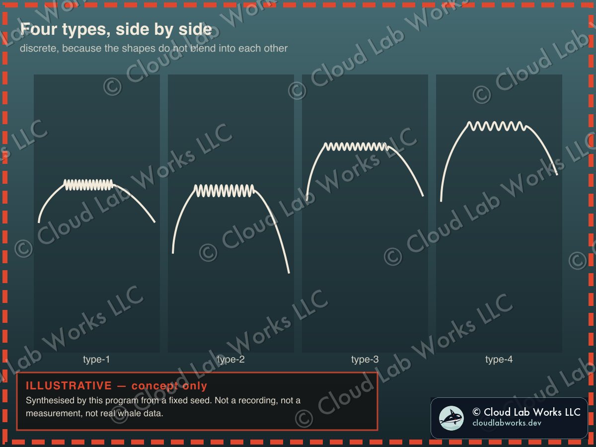 SVG · Call catalogue · illustrativeFour types, side by sideFour contours from seeds 101–104. Plateau-to-terminal drop ranges 366–775 Hz across the set. Discreteness is the claim worth keeping: types are countable, which is what makes acoustic identification possible at all.Inquire
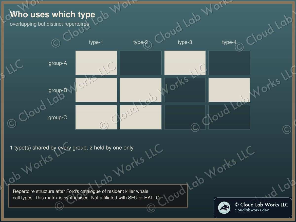 SVG · Call catalogue · sourcedWho uses which type3 groups × 4 types, seed 7: 1 type(s) used by every group, 2 held by exactly one. The idea that pods hold overlapping-but-distinct repertoires is Ford’s and is credited on the card; this particular matrix is program output.Inquire
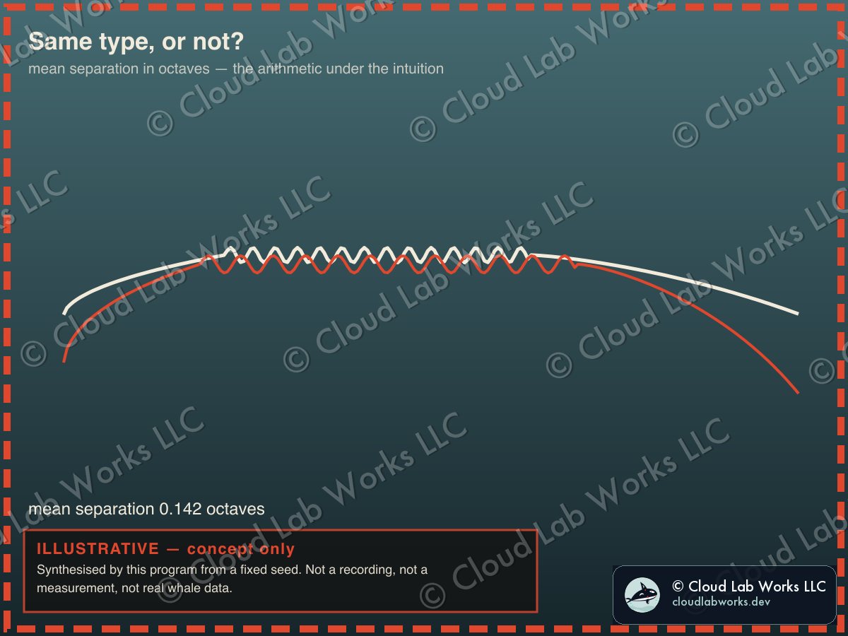 SVG · Call catalogue · illustrativeSame type, or not?Contour 101 against contour 102: 0.142 octaves mean separation, against 0.000 for a contour matched with itself. A real classifier does far more than this — HALLO’s is a neural one — but this is the quantity the intuition is reaching for.Inquire
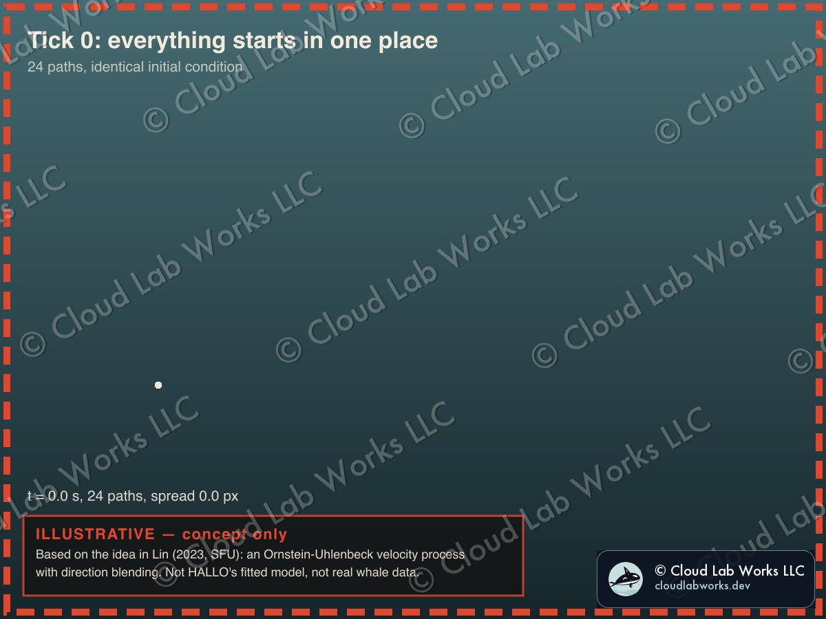 SVG · Forecast · illustrativeTick 0: everything starts in one placet = 0.0 s, tick 0 of 300. Ensemble spread 0.0 px around a centroid at (230, 560). θ = 0.55, σ = 14.0, preferred cruise 42.0 px/s, heading blend 0.72/0.28.Inquire
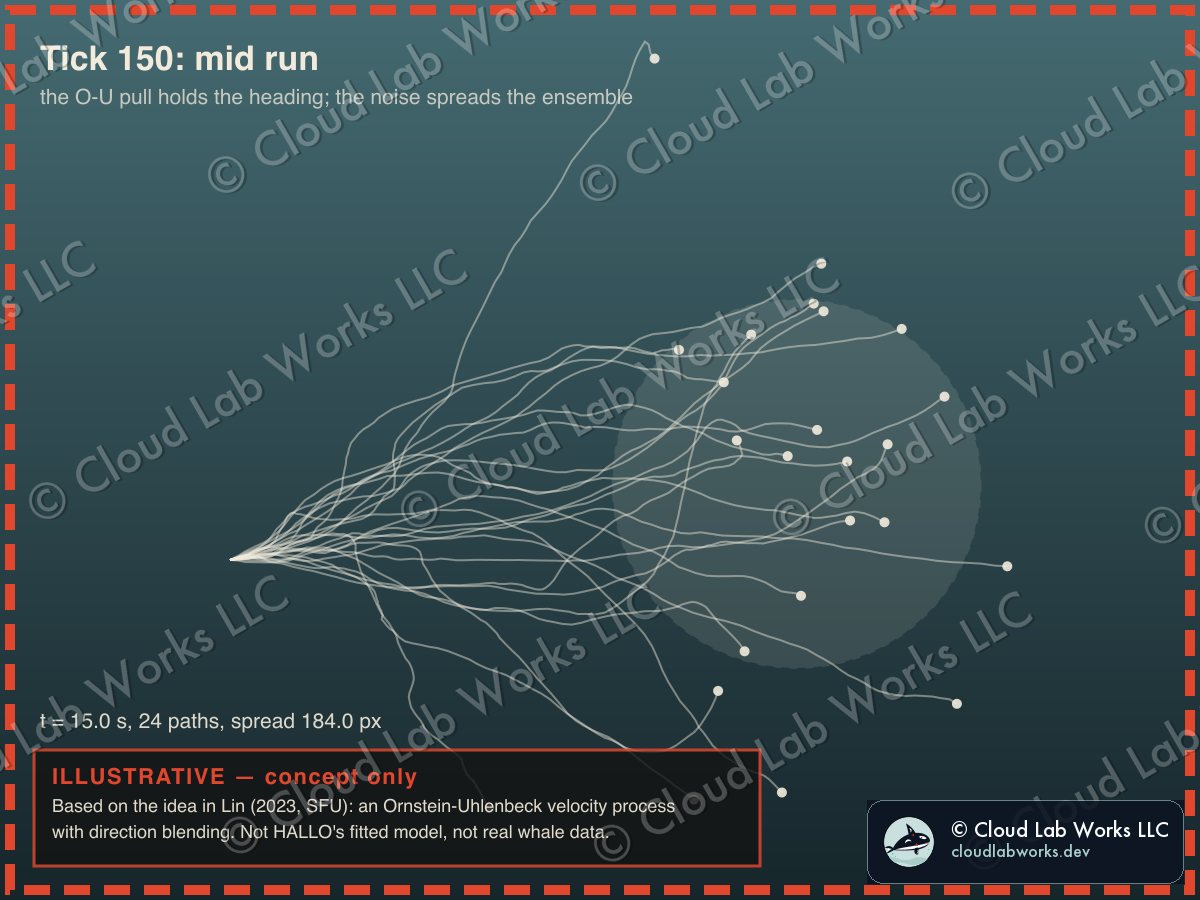 SVG · Forecast · illustrativeTick 150: mid runt = 15.0 s, tick 150 of 300. Ensemble spread 184.0 px around a centroid at (797, 484). θ = 0.55, σ = 14.0, preferred cruise 42.0 px/s, heading blend 0.72/0.28.Inquire
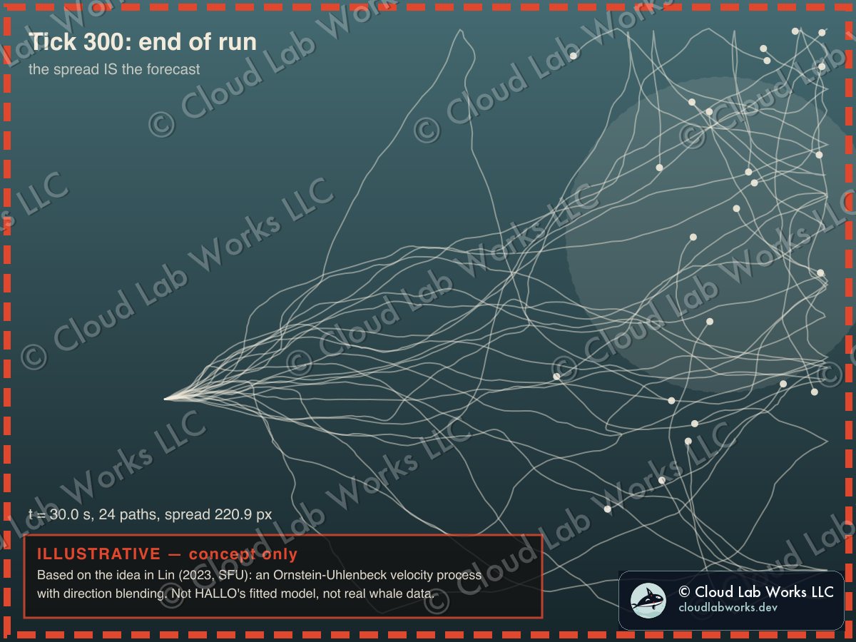 SVG · Forecast · illustrativeTick 300: end of runt = 30.0 s, tick 300 of 300. Ensemble spread 220.9 px around a centroid at (1014, 329). θ = 0.55, σ = 14.0, preferred cruise 42.0 px/s, heading blend 0.72/0.28.Inquire
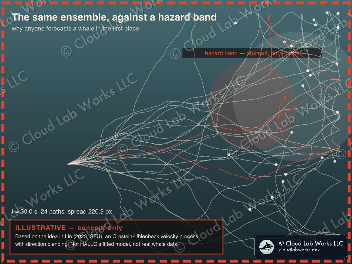 SVG · Forecast · illustrativeThe same ensemble, against a hazard band2 of 24 paths end inside the band at t = 30.0 s. The band is a circle on an empty field on purpose: it is not a channel, not a shipping lane, not a map of anywhere. The output of a real system is a probability over a real place, and this is not one.Inquire
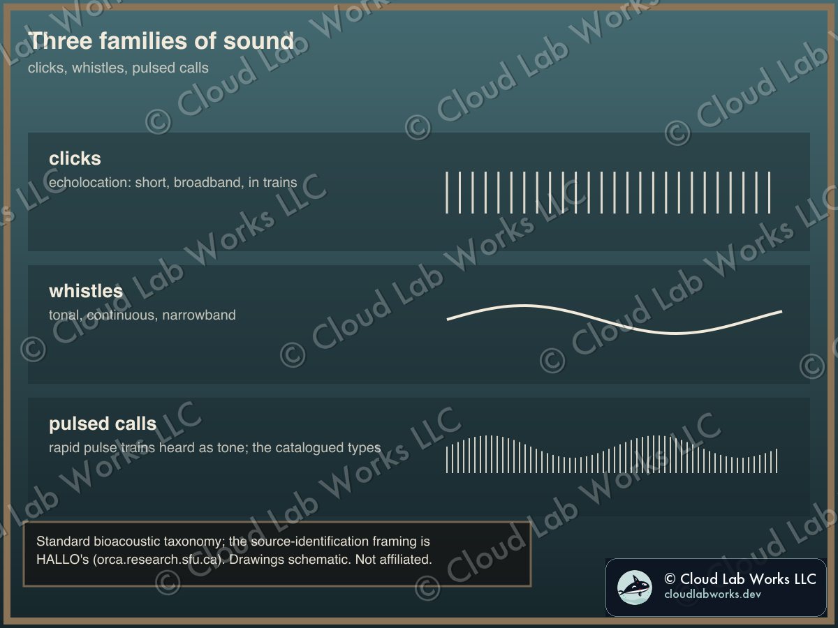 SVG · Bioacoustics · sourcedThree families of soundClicks for echolocation, whistles for tonal contact, pulsed calls for the catalogued repertoire. Standard taxonomy, credited on the card; the drawings are schematic, and the source-identification framing is HALLO’s. Not affiliated with SFU or HALLO.Inquire
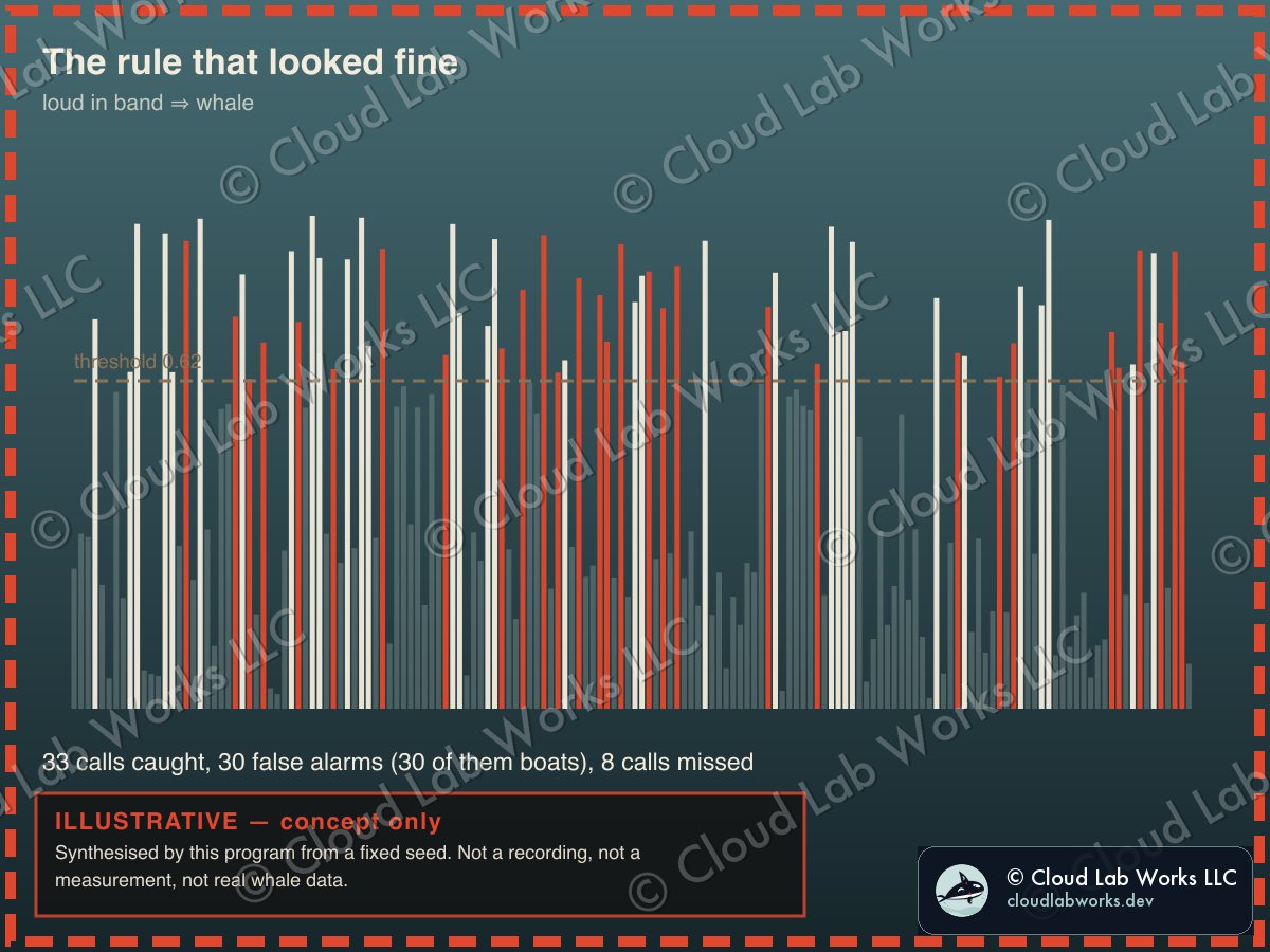 SVG · Bioacoustics · illustrativeThe rule that looked fine160 synthetic events at threshold 0.62: 33 calls caught, 30 false alarms of which 30 are boats, 8 calls missed. A boat is loud in band too. This is the card that replaced a confusion matrix, because a matrix reads as a result no matter what the caption underneath it says.Inquire
Watermarked like everything on Code as Art; the SVG originals stay in the repo's source tree. Inquire for a print or the source of a card.
state.json as gen.py wrote it: every parameter and every measured number the page is allowed to quote.
{
  "calls": {
    "contours": {
      "seed-101": {
        "seed": 101,
        "dur_s": 1.6,
        "f_onset": 890.5760662522823,
        "f_plateau": 1260.6472214554312,
        "f_terminal": 894.5241708482918,
        "wobble_hz": 8.543858410060766,
        "wobble_frac": 0.0433569339098487
      },
      "seed-102": {
        "seed": 102,
        "dur_s": 1.6,
        "f_onset": 674.0856031935418,
        "f_plateau": 1195.5383362642276,
        "f_terminal": 562.9858729657519,
        "wobble_hz": 7.275041684251246,
        "wobble_frac": 0.05039162463787357
      },
      "seed-103": {
        "seed": 103,
        "dur_s": 1.6,
        "f_onset": 1089.5250600363872,
        "f_plateau": 1784.4824708861536,
        "f_terminal": 1134.3136172522964,
        "wobble_hz": 7.409317455512037,
        "wobble_frac": 0.03074508342485317
      },
      "seed-104": {
        "seed": 104,
        "dur_s": 1.6,
        "f_onset": 1079.9804650974777,
        "f_plateau": 2150.331969052251,
        "f_terminal": 1375.291233079216,
        "wobble_hz": 4.365734445647711,
        "wobble_frac": 0.03653211638582625
      }
    },
    "distance_101_102_octaves": 0.1418,
    "distance_self_octaves": 0,
    "repertoire": {
      "seed": 7,
      "labels": [
        "group-A",
        "group-B",
        "group-C"
      ],
      "names": [
        "type-1",
        "type-2",
        "type-3",
        "type-4"
      ],
      "grid": [
        [
          true,
          false,
          true,
          false
        ],
        [
          true,
          true,
          false,
          true
        ],
        [
          true,
          true,
          false,
          false
        ]
      ],
      "shared": 1,
      "unique": 2
    }
  },
  "forecast": {
    "theta": 0.55,
    "sigma": 14,
    "mu_speed": 42,
    "w_persist": 0.72,
    "w_prefer": 0.28,
    "seed": 3,
    "n_paths": 24,
    "ticks": 300,
    "dt_s": 0.1,
    "hazard": {
      "x": 860,
      "y": 360,
      "r": 150
    },
    "frames": {
      "0": {
        "tick": 0,
        "t_s": 0,
        "spread_px": 0,
        "centroid": [
          230,
          560
        ],
        "in_hazard": 0
      },
      "150": {
        "tick": 150,
        "t_s": 15,
        "spread_px": 184,
        "centroid": [
          796.6,
          483.9
        ],
        "in_hazard": 12
      },
      "300": {
        "tick": 300,
        "t_s": 30,
        "spread_px": 220.9,
        "centroid": [
          1014.3,
          329.1
        ],
        "in_hazard": 2
      }
    },
    "final_state": {
      "tick": 300,
      "t_s": 30,
      "spread_px": 220.9,
      "centroid": [
        1014.3,
        329.1
      ],
      "in_hazard": 2
    }
  },
  "detector": {
    "seed": 5,
    "n": 160,
    "threshold": 0.62,
    "true_positive": 33,
    "false_positive": 30,
    "false_negative": 8,
    "boat_fires": 30
  },
  "badges": {
    "forecast": [
      "ILLUSTRATIVE — concept only",
      "Based on the idea in Lin (2023, SFU): an Ornstein-Uhlenbeck velocity process",
      "with direction blending. Not HALLO's fitted model, not real whale data."
    ],
    "synthetic": [
      "ILLUSTRATIVE — concept only",
      "Synthesised by this program from a fixed seed. Not a recording, not a",
      "measurement, not real whale data."
    ]
  },
  "credits": {
    "ford": "Repertoire structure after Ford's catalogue of resident killer whale call types. This matrix is synthesised. Not affiliated with SFU or HALLO.",
    "families": "Standard bioacoustic taxonomy; the source-identification framing is HALLO's (orca.research.sfu.ca). Drawings schematic. Not affiliated."
  },
  "counts": {
    "total": 10,
    "call_catalogue": 4,
    "forecast": 4,
    "bioacoustics": 2,
    "sourced": 2,
    "illustrative": 8
  }
}
Credits, and what they are not
The HALLO project at Simon Fraser University is the reason this page has a frame to hang on: a classifier posed as source identification rather than mere detection, with models open-sourced and ecotype and pod-level work ahead of it. Lin (2023, SFU) is the thesis whose Ornstein-Uhlenbeck velocity process with direction blending the forecast cards illustrate the idea of. John Ford's catalogue of resident call types is why "discrete repertoire per pod" is a real structure and not one invented here. Citations verified against the live sources; none of these people or institutions has reviewed, endorsed, or is connected to this page.
The Southern Resident population these methods exist to help is down to a number small enough to list by name. That is the actual subject, and it is the reason the disclaimers on this page are heavy rather than decorative: work about an endangered animal is exactly where a pretty synthetic picture mistaken for a measurement does real harm.
Next rungs, in order: a real spectrogram path — synthesis first, so there is still no recording in the tree — then a contour-matching pass that reports its errors the way the detector card does. Further out, the honest blocker: everything above is a drawing of a method, and the difference between drawing one and running one is the whole of the work. Nothing on this page should be cited as a result, and it is built so that it cannot be mistaken for one at a glance.